Database changes have finished applying - please report any issues you're (still) seeing to support@shoutwiki.com.
- Previous: Chapter 5 - Loads
- Next: Chapter 7 - Advanced Distribution Models
GridLAB-D provides models for several different types of distributed generation assets including diesel and wind but for this tutorial we’re going to focus on the the increasingly important solar PV generators and batteries.
Solar PV
The solar PV class in GridLAB-D uses the solar parameters from the climate object in the model and the parameters specified in the object itself to generate a DC power value. To tie into the rest of the GridLAB-D simulation, this DC power needs to be converted to an AC value, either split phase as for a “house” object or three-phase for general distribution node. The solar PV class has parameters that are closer to first-principles than power engineers may be used to; instead of specifying a 5 kW installation the class asks for panel type, square-footage of the installation, efficiency, and normal operating cell temperature, among others.
Being so closely tied to the physics of the system, the model relies on three solar parameters to correctly calculate the effective solar radiation that is used by the panel to produce electrical energy. These values are defined in the climate object which must be included in the model (.glm); typically they are provided by TMY data though they could alternatively be defined with player files using an external data source.
There are two types of solar models used in GridLAB-D: a solar tilt model and a solar power model. The tilt model is used to calculate the amount of solar radiation striking the face of the solar panel. GridLAB-D has two models, the default (based on B. Y. H. Liu and R. C. Jordan, “The interrelationship and characteristic distribution of direct, diffuse and total solar radiation,” Solar Energy, vol. 4, no. 3, pp. 1–19, 1960.) and SOLPOS; SOLPOS is used in NREL's PVWatts, has been validated against it, and is the preferred model.
The solar power model takes the power generated in the tilt model and adjusts it based on the thermal parameters of the solar panel. There are two power models in GridLAB-D, the default and the FLATPLATE, the later contains a more complex thermal model and is the slightly preferred model to use because of this.
Inverters
Since a solar PV installation is inherently DC and the electrical grid is AC, an inverter is needed to connect the two. The inverter is assumed to provide ideal maximum power-point tracking, able to convert the maximum power from the solar installation that is supported by the conditions at a given point in time. When the inverter is commanded to produce less than this power it is assumed the solar PV panel is loaded in such a way as to provide this power and the potential power output of the panel is not fully realized.
As of the time of this writing, the inverter model is a mix of older legacy code that will likely be deprecated in the near future and newer, active development and maintenance code. The most up-to-date model sets the inverter_type to FOUR_QUADRANT; though this model has several different control modes, most don't work properly with solar panels. Leaving the four_quadrant_control_mode parameter unspecified (that is, not including it in the parameter definitions for that object), will default to an operating mode that transfers the maximum real energy possible from the solar panel at all times. We'll discuss some of the other operating modes of the inverter when we cover energy storage later on in this chapter.
Example - Basic Solar PV Installation
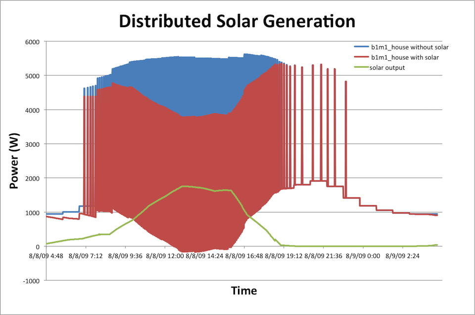
The file dist_gen_solar_single.glm [1] contains the feeder model we've been using up to this point with a single added solar installation. Measuring the net power flow at b1m1_house_node, upstream of both the solar PV installation, its inverter, and the house load itself, we can see that the impact that the solar PV installation has on the total residential load. During some portion of the day, when the air-conditioner is off the solar power output is greater than the house load, leading to reverse power flow back into the distribution system.
Example - Large Solar PV Installation and Impact on Feeder
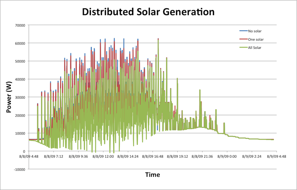
The file dist_gen_solar_all.glm [2] takes uses the same architecture and adds solar PV installations to all the houses on our small feeder model. Looking at the total power flow up at the feeder head, we can see that adding solar power to each of the houses dramatically reduces the total feeder load during the sunny part of the day, again leading to a few moments where the total feeder power is negative. During these times the feeder is effectively acting as a generator and feeder power back to the bulk power system as a whole (which we haven't included in our model).
Battery Energy Storage
Confusingly, GridLAB-D contains two classes that both look like they could be used for adding energy storage to a GridLAB-D model: energy_storage and battery. A quick look at the energy_storage wiki page and source code reveals that this class type is not fully implemented forcing us to use the battery class instead. Unfortunately, like the inverter class, there is a mix of legacy and modern code and models. The most modern and maintained branch of this class sets use_internal_battery_model to TRUE. This enables a simple battery model with only a few parameters such as efficiency and energy and power ratings.
The bulk of the capability when using the battery model comes from the inverter that is paired with it. Again, just like we did with the solar panel, setting inverter_type to FOUR_QUADRANT uses the most current model and unlike with a solar PV installation, the four_quadrant_control_mode parameter is fully functional and opens up a wide variety of control modes.
- CONSTANT_PQ - Sets the output of the battery to the specified constant real and reactive power levels. This mode in particular lends itself to using player files or schedules to control the battery, allowing the charge and discharge time to be scheduled.
- CONSTANT_PF - This is the default controller mode with the power factor set to unity. With a solar panel installation this works wonderfully as the inverter will generate as much real power as the panel provides. (xxxxxxx Can charging and discharging be controlled? It doesn't look like it based on the code.)
- VOLT_VAR - Uses the reactive power capability of the inverter to regulate the voltage at the point of common coupling. This mode allows the user to input a voltage vs reactive power curve to define how aggressively the inverter attempts to regulate the voltage.
- LOAD_FOLLOWING - Allows the inverter to use the energy from the battery to regulate the load at a user-definable point on the feeder. The user defines a charge/discharge hysteresis curve to dictate how the battery/inverter combination will operate.
Example - Load-Following for a Single Residence
As an example of how to use a battery in GridLAB-D, we are going to demonstrate how to use the inverter load-following mode, a mode that uses an energy storage device to peak-shave and valley-fill the load at a specified point in the distribution feeder. The model file is dist_gen_load_following.glm [3] and it has been changed by:
- Adding module generators to the list of specific modules GridLAB-D needs to load as a part of running a simulation of this model.
- Installing a separate triplex line and meter on b1m1 so that the energy from the battery can be uniquely measured and not conflated with the load from the house.
- Installing the inverter and battery on downstream of the new triplex line and meter.
- To support the LOAD_FOLLOWING mode on the inverter we need to define a node upstream of the inverter and house that will be used as a reference point. We already had a node (b1m1_house_node) and changing it to a meter will open up some measurement parameters that will be convenient to use.
With the new objects added to the model, the only tricky part now is setting up the LOAD_FOLLOWING mode correctly in the object parameter list. LOAD_FOLLOWING works by charging when the reference load is low enough and discharging when that load is too high. To add extra flexibility, hysteresis is included; for example, charge_on_threshold is power below which the inverter will begin to charge the battery and charge_off_threshold is the power above which the inverter will stop charging the battery. Since this is a hysteresis operation, charge_on_threshold must be lower than charge_off_threshold. A similar definition exists for the discharge operation when the load gets too high.
The power levels that the inverter will reference in making these control decisions are defined by the sense_object parameter. This object must be upstream of the inverter; that is, the power produced by the inverter must flow through this meter for LOAD_FOLLOWING to work. Lastly, a pause time in seconds between the end of the charge and discharge operation (charge_lockout_time and discharge_lockout_time , respectively) can also be defined.
Running this simulation produces a few warnings (not errors, which would halt the simulation). The first is a reminder that in LOAD_FOLLOWING, the sense_object must be upstream, as previously discussed.
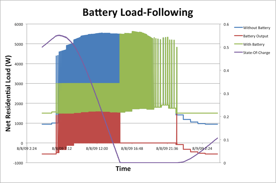
Looking at the file b1h1_house_data.csv [4] and comparing it to how the system behaved prior to the installation of the battery and inverter, we can see that the load-following is set-up correctly to fill the low points in the residential load and shave the peaks when that load gets too high.
Except not all the time. Towards the end of the day we can see that the state-of-charge of the battery reaches zero, at which point it is no longer able to discharge, eliminating its ability to shave the peak. The battery stays in this depleted state until the load at the reference meter falls below the charge_on_threshold value of 1.5 kW, at which point the battery begins to charge, partially restoring the state of charge. Compared to where the battery started the day though, the ending state-of-charge is pretty low and its easy to see that attempts to shave the peak on the following day probably will also fall short, perhaps even earlier in the day.
Example - Solar PV and Battery Combination
Combining solar PV and energy storage can create an effective solution for regulating the load. The model defined in the file dist_gen_battery_solar.glm [5] has such an example. To the same house that already had energy storage installed, a solar PV installation was added. As before, it is the inverter that controls the power flow from the solar panels and the control mode chosen CONSTANT_PF defaults to only producing real power, passing all the available energy generated by the solar PV installation onto the grid.
You'll also notice that the solar PV installation has its own triplex line, meter and inverter. Despite the fact that it generally possible to connect solar panels and batteries to the same inverter in real-world installations, GridLAB-D has no solver for DC powerflow and thus requires separate AC connections through inverters. This doesn't mean that the solar panels won't charge the batteries, we'll see that they do in a moment. Rather, it means that the energy flows through the AC network and as a consequence, is available for separate metering.
Looking at the definition of the solar object, you'll see that the parameters provided are derived from a physics-level perspective. Area of solar panel installation, efficiency, panel type, panel orientation, power production models (among others), all are used to define how this installation will generate energy as the solar conditions change throughout the day (and year). This particular installation produces more than 1 kW during peak solar conditions.
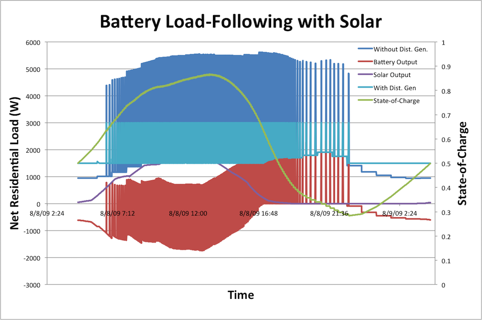
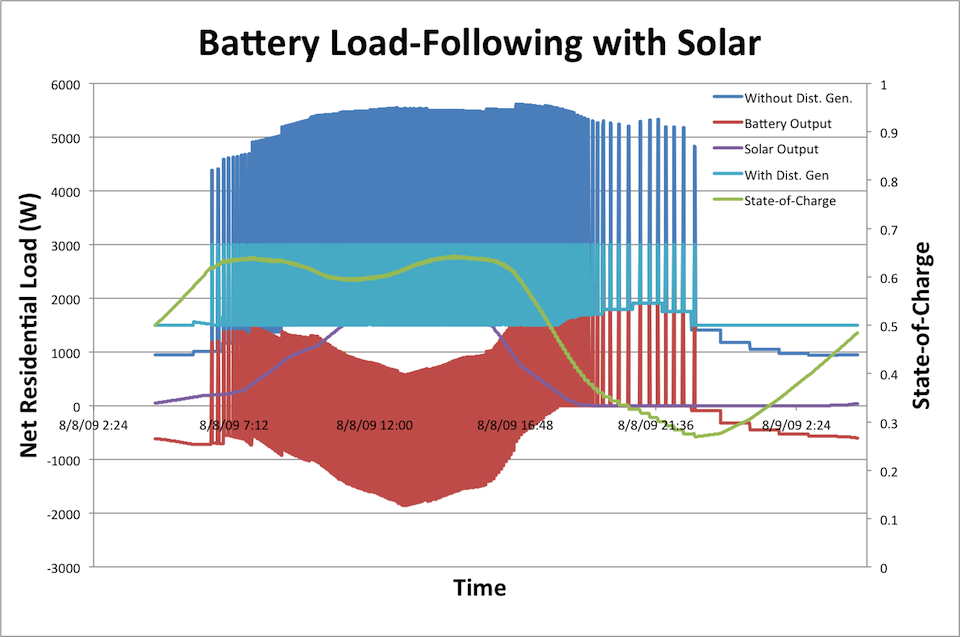
Running this simulation and looking at the data in the file b1h1_house_data.csv [6] shows that the addition of solar greatly increases the effectively of the peak-shaving. Not only does the battery get close to full capacity before called-on mid-morning, the battery is far from empty when the end of the peak-shaving activity for the day is over, using only a third of its capacity. By having the energy storage work in parallel with the solar PV installation, the early morning solar energy production is effectively stored for use later in the day when it is needed to limit the demand of this residential load.
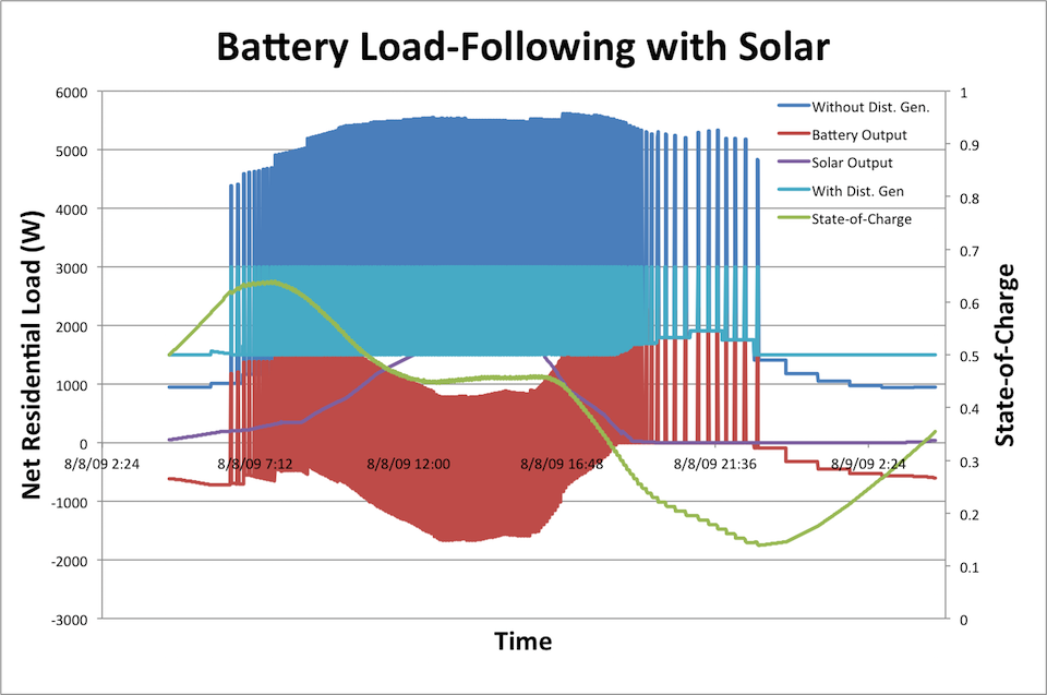
If we wanted to try to align the peak of the solar generation better with the peak of the residential load we can change the orientation of the solar PV panels so that they are pointed more southwest, rather than directly south. Change the orientation_azimuth to 230 and re-run the simulation.
Adjusting the angle again so the panels face directly west produces the following:
A few important notes from this:
- Total solar energy output - 14.1 kWh generated when facing southwest vs 14.4 kWh when facing directly south and 12.9 kWh when facing directly west.
- Total net battery energy transacted - 1.5 kWh of net load when facing southwest vs 1.9 kWh when facing directly south and 0.25 kWh when facing directly west.
As the panel points more and more westward, the total solar energy production goes down and its ability to recharge the battery is reduced. The big advantage of facing somewhat westward, though, is that it tends to line up the load on the system as air-conditioners run heavily in the late afternoon and early evening. This is particularly beneficial for residential customers that pay different rates during different times of the day but that gets into the economics of energy and that we won't get into that right now.
- Previous: Chapter 5 - Loads
- Next: Chapter 7 - Advanced Distribution Models
